Sensor Fusion
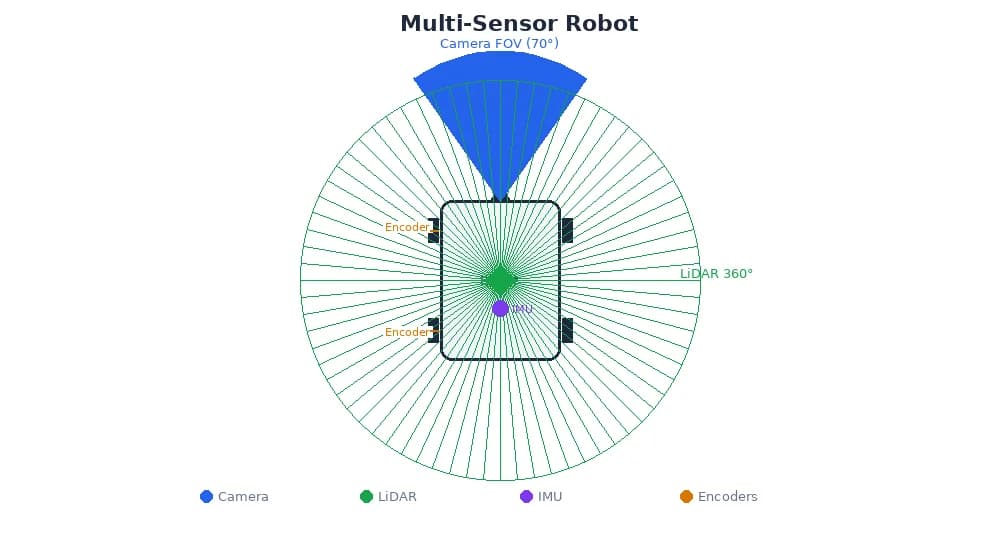
No single sensor tells the whole story. Cameras see rich detail but lack depth. LiDAR measures distance precisely but has no color. IMUs track motion but drift over time. Sensor fusion combines multiple sensors to get a better picture than any one sensor alone.
Why Combine Sensors?
Each sensor has strengths and weaknesses:
| Sensor | Strengths | Weaknesses |
|---|---|---|
| Camera | Rich texture, color, high resolution | No depth, fails in darkness |
| LiDAR | Precise 3D geometry, works in darkness | No color/texture, expensive |
| IMU | High-frequency motion updates | Drifts over time, no absolute position |
| GPS | Absolute global position | 1-5m error, doesn't work indoors |
| Wheel Encoders | Smooth short-term motion | Accumulates error (wheel slip, drift) |
Fusion compensates for each sensor's weaknesses:
- Camera + LiDAR: 3D bounding boxes with visual classification
- IMU + GPS: Smooth trajectory with absolute position correction
- Wheel encoders + IMU: Accurate short-term odometry, corrected by periodic landmarks
Self-driving cars use camera + LiDAR + radar + GPS + IMU. Redundancy is critical — if LiDAR fails (heavy rain), cameras and radar keep the car safe. If GPS drops out (tunnel), IMU and odometry maintain position until GPS returns.
Early vs. Late Fusion
Two fundamental strategies for combining sensors:
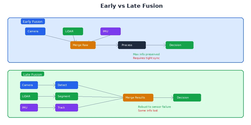
Early Fusion (Sensor-Level)
Combine raw data before processing:
- Align camera and depth images pixel-by-pixel
- Merge LiDAR points with camera colors
- Create a unified representation (e.g., colored point cloud)
Pros:
- Maximum information preserved
- More accurate when sensors are perfectly aligned
Cons:
- Requires tight synchronization
- Calibration is critical (misalignment ruins everything)
- Computationally expensive
# Combine RGB camera + depth camera into colored point cloud
rgb_image = camera.capture()
depth_image = depth_camera.capture()

points = []
for y in range(height):
    for x in range(width):
        z = depth_image[y, x]
        if z > 0:  # valid depth
            # Unproject to 3D
            X = (x - cx) * z / fx
            Y = (y - cy) * z / fy
            Z = z

            # Get color from RGB image
            r, g, b = rgb_image[y, x]

            points.append({
                "position": (X, Y, Z),
                "color": (r, g, b)
            })

# Now you have a point cloud with full color and geometry
Late Fusion (Decision-Level)
Process each sensor independently, then combine results:
- Camera detects "person" at pixel (320, 240)
- LiDAR measures distance 2.5m at that angle
- Combine: "person at (x=2.5m, y=0, z=0)"
Pros:
- Each sensor can run at its own rate
- Easier to handle sensor failures (just drop that input)
- More modular — swap sensors without rewriting the whole pipeline
Cons:
- Information loss (each sensor's pipeline makes irreversible decisions)
- Harder to resolve conflicts (camera says "person", LiDAR says "empty")
# Camera: detect objects
detections = yolo_detector.run(rgb_image)
# Result: [{"class": "person", "bbox": (120, 50, 80, 200), "confidence": 0.92}]

# LiDAR: get distance at detection center
for det in detections:
    cx = det["bbox"]["x"] + det["bbox"]["width"] / 2
    cy = det["bbox"]["y"] + det["bbox"]["height"] / 2

    # Get depth at that pixel (from aligned depth camera or projected LiDAR)
    depth = depth_image[int(cy), int(cx)]

    # Unproject to 3D
    X = (cx - camera_cx) * depth / camera_fx
    Y = (cy - camera_cy) * depth / camera_fy
    Z = depth

    det["position_3d"] = (X, Y, Z)

# Now detections have 3D positions!For robotics, late fusion is more common — it's robust to sensor timing differences and easier to debug. Early fusion is used when you need the absolute best accuracy (e.g., 3D reconstruction, precision manipulation).
The Kalman Filter: Fusion in Motion
When tracking moving objects (or your own robot's position), you need to handle:
- Noisy measurements — sensors aren't perfect
- Predictions — where will the object be next?
- Updates — how do we correct the prediction when new data arrives?
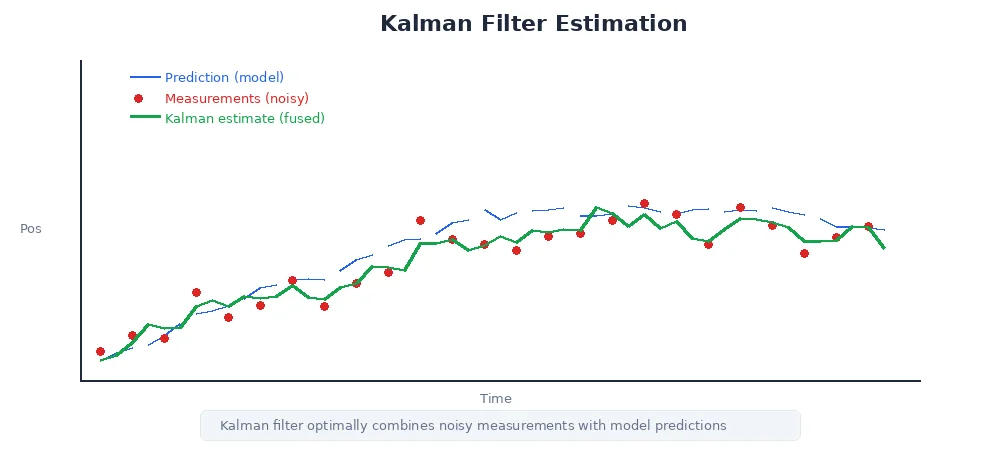
The Kalman filter is the standard solution. It's a recursive algorithm that:
- Predicts the next state using a motion model
- Updates the prediction using new sensor data
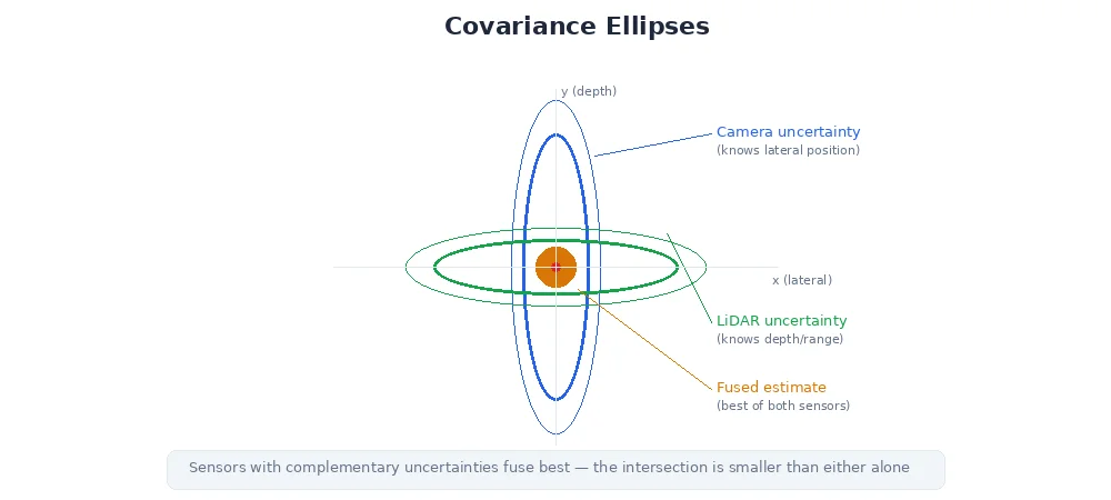
- Weights the prediction vs. measurement based on their uncertainties
Kalman Filter Example: Tracking a Ball
# State: position and velocity
position = 0.0
velocity = 0.0

# Uncertainties (how much we trust our estimate)
position_uncertainty = 1.0
velocity_uncertainty = 1.0

# Process noise (things we can't predict: wind, friction)
process_noise = 0.1

# Measurement noise (sensor error)
measurement_noise = 0.5

# Prediction step (physics)
dt = 0.1  # time step
position = position + velocity * dt
position_uncertainty += process_noise

# Update step (sensor measurement)
measured_position = camera.get_ball_position()  # e.g., 1.2m

# Kalman gain: how much to trust the measurement
K = position_uncertainty / (position_uncertainty + measurement_noise)

# Fuse prediction + measurement
position = position + K * (measured_position - position)
position_uncertainty = (1 - K) * position_uncertainty

# Now 'position' is the best estimate combining physics + sensor
The beauty: if the sensor is noisy (high measurement_noise), the filter trusts the prediction more. If the model is uncertain (high process_noise), it trusts the sensor more. Optimal fusion automatically.
Practical Sensor Fusion Examples
1. Camera + LiDAR for Object Detection
- Camera: Detect "car" with 2D bounding box
- LiDAR: Measure point cloud in that bbox region
- Fusion: Fit 3D bounding box to LiDAR points, label it "car"
- Result: 3D position, orientation, and size of the car
2. GPS + IMU for Drone Localization
- GPS: Noisy absolute position, 1 Hz
- IMU: Clean acceleration/rotation, 100 Hz
- Fusion (Kalman): Integrate IMU for smooth high-frequency position, correct with GPS every second
- Result: 100 Hz position updates with GPS-level long-term accuracy
3. Stereo Camera + Wheel Odometry for Navigation
- Wheel encoders: Fast, smooth motion estimates (but drift over time)
- Stereo camera: Slow, precise position from visual landmarks
- Fusion: Use odometry between landmark observations, reset drift when landmarks are detected
- Result: Accurate position even during fast motion or wheel slip
What's Next?
You've now learned the fundamentals of robot perception — cameras, LiDAR, depth sensing, object detection, and sensor fusion. In the next module, we'll explore localization and mapping — how robots figure out where they are and build maps of their environment using these sensors.