Finding Yourself on a Known Map

You wake up in a large hotel. You know you're somewhere on the fifth floor, but which hallway? You look around — there's a fire extinguisher on the wall, an exit sign, and a door marked "503." By combining these observations with the floor plan, you quickly figure out exactly where you are.

That's localization. The robot has a map and needs to answer one question: where am I on this map?

The Localization Problem

Localization might sound easier than mapping — after all, the map is already known. But it has its own challenges:

Initial Position Uncertainty

Sometimes the robot knows roughly where it started. Other times (called "global localization" or the "kidnapped robot problem"), it has no idea. Imagine being teleported to a random hallway — you'd need to look around and match features to the map.

Sensor Ambiguity

Many places look similar. One hallway intersection looks just like another. The robot's sensors might match multiple locations on the map.

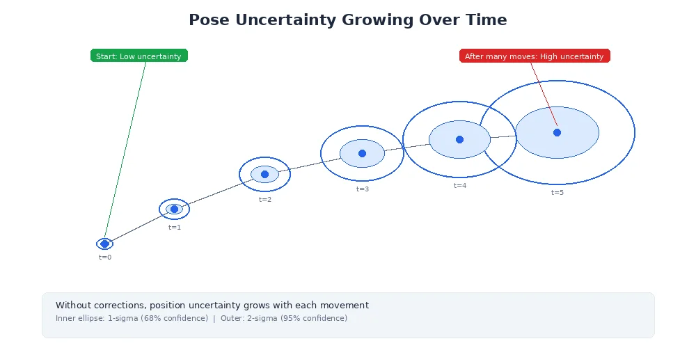
Pose uncertainty ellipse — showing how position uncertainty grows over time as the robot moves without corrections — As the robot moves, its position uncertainty grows like an expanding ellipse. The ellipse is narrow in the direction of travel (encoders are decent) but wide perpendicular to it (lateral drift is hard to detect). Landmarks shrink the ellipse back down.

Motion Uncertainty

As the robot moves, wheel slippage and uneven floors introduce errors. The robot thinks it moved 1 meter forward but actually moved 0.98 meters. These errors accumulate.

Warning

Localization is only as good as the map. If the map is outdated (furniture moved, walls added), the robot will struggle to figure out where it is because its sensor readings won't match the map.

The Particle Filter Solution

The most popular localization approach is called Monte Carlo Localization (MCL), which uses a particle filter. Here's the core idea:

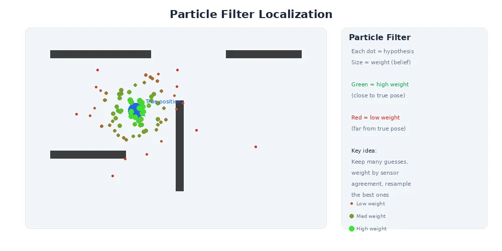
Particle filter visualization — thousands of particles converging from a scattered cloud to a tight cluster around the true position — A particle filter starts with particles scattered across the map (high uncertainty). After several motion-and-sensing cycles, particles in wrong locations die off and particles near the true position multiply, forming a tight cluster.

Instead of tracking a single "I think I'm here" guess, the robot maintains thousands of particles — each particle is a hypothesis about where the robot might be. Over time, particles in wrong locations die off, and particles in correct locations multiply.

Think of it like evolution: hypotheses compete, and the fittest (those that best match sensor observations) survive.

How Particle Filters Work

Here's the step-by-step process:

1. Initialize Particles

Scatter thousands of particles randomly across the map (or around a known starting area). Each particle represents a possible robot pose (x, y, orientation).

2. Motion Update (Prediction)

When the robot moves, move all particles according to the same motion command — but add noise. If the robot drove forward 1 meter, each particle moves forward 1 meter ± a small random error. This reflects the uncertainty in real robot motion.

3. Sensor Update (Measurement)

When sensors take a reading (LiDAR scan, camera image), compare what each particle would see from its hypothetical position against what the robot actually saw. Particles whose predicted observations match reality get higher weights (more "fitness").

4. Resampling

Randomly draw a new set of particles, where particles with higher weights are more likely to be selected multiple times. Low-weight particles (bad hypotheses) usually disappear.

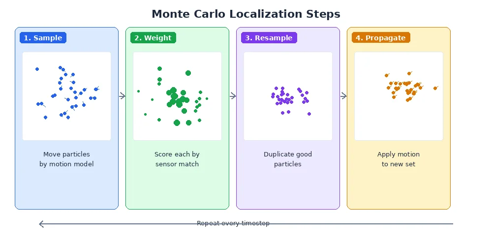
MCL algorithm steps — showing the four phases: initialize, predict (motion), update (sensor), and resample — Monte Carlo Localization repeats four steps in a loop: (1) spread particles, (2) move them according to odometry + noise, (3) weight them by how well their predicted sensor readings match reality, (4) resample — keeping high-weight particles and discarding low-weight ones.

5. Repeat

As the robot moves and gathers more sensor data, the particle cloud converges on the true position.

Particle Filter Pseudocode

particles = initialize_random_particles(map, count=1000)
 
while robot_is_running:
    # Robot moves
    motion = get_odometry_update()
    for particle in particles:
        particle.pose = apply_motion(particle.pose, motion, noise)
 
    # Robot senses
    sensor_data = get_lidar_scan()
    for particle in particles:
        expected = predict_scan(particle.pose, map)
        particle.weight = similarity(sensor_data, expected)
 
    # Resample based on weights
    particles = resample_weighted(particles)
 
    # Best estimate = weighted average of particles
    estimated_pose = compute_mean(particles)

Why Particles Beat Single-Guess Tracking

Imagine a robot in a symmetric hallway. Its sensors say "I see walls to my left and right, open space ahead." That matches four possible locations. A single-hypothesis tracker would have to pick one and hope it's right. A particle filter keeps all four hypotheses alive until new evidence (like seeing a specific doorway) disambiguates.

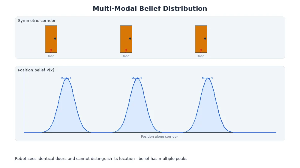
Multi-modal belief distribution — showing particle clusters at multiple possible positions that converge as the robot observes more landmarks — In a symmetric environment, particles cluster at multiple possible positions (multi-modal belief). As the robot moves and observes unique landmarks, wrong hypotheses lose particles until only the correct cluster remains.

This is called multi-modal belief — the robot's belief has multiple "peaks" of probability until more information narrows it down.

Tip

You can visualize particle filters by plotting particles on the map. A tight cluster means high certainty. A spread-out cloud means the robot is uncertain and needs more distinctive landmarks.

The Importance of Distinctive Features

Localization works best when the environment has distinctive, unambiguous features:

Unique furniture arrangements
Recognizable landmarks (a fire extinguisher, a specific poster)
Asymmetric room layouts

Long, featureless hallways are localization nightmares. If every meter looks identical, the robot can't tell if it's moved. That's why airports and hospitals often add visual markers to help human navigation — robots benefit from the same thing.

Recovery from Failures

Sometimes localization fails completely — maybe the robot got pushed, or a door closed and blocked a familiar landmark. Good localization systems detect when the particle cloud becomes too spread out and trigger recovery behaviors:

Spin in place to gather 360° of sensor data
Move to a known distinctive landmark
Temporarily increase particle count to explore more hypotheses

What's Next?

Mapping requires knowing where you are. Localization requires having a map. So what happens when you have neither? That's the famous SLAM problem — Simultaneous Localization And Mapping — and it's the topic of our next lesson.

Localization Basics