Grid-Based Planning
Take a map. Divide it into a grid. Mark each cell as "free" or "blocked." Now find the shortest path from start to goal.
This is grid-based planning, and it's the foundation of most 2D robot navigation. The algorithm at its core? A* (A-star) — a search algorithm so elegant it's taught in every computer science course.
Occupancy Grids
An occupancy grid is a 2D array representing the world. Each cell stores a probability: "How certain am I that this space is occupied?"
    0   1   2   3   4   5
  ┌───┬───┬───┬───┬───┬───┐
0 │ 0 │ 0 │100│100│100│ 0 │   0 = free
  ├───┼───┼───┼───┼───┼───┤  100 = occupied
1 │ 0 │ 0 │100│ 0 │ 0 │ 0 │   50 = unknown
  ├───┼───┼───┼───┼───┼───┤
2 │ S │ 0 │100│ 0 │ 0 │ G │   S = start, G = goal
  ├───┼───┼───┼───┼───┼───┤
3 │ 0 │ 0 │ 0 │ 0 │ 0 │ 0 │
  └───┴───┴───┴───┴───┴───┘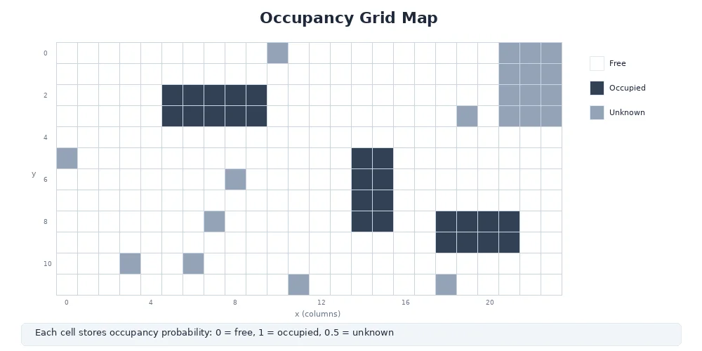
Each cell might be 5cm × 5cm (high resolution) or 10cm × 10cm (coarser, faster). The grid resolution is a key trade-off:
| Resolution | Pros | Cons |
|---|---|---|
| Fine (5cm) | Accurate, finds narrow paths | Large memory, slow search |
| Coarse (20cm) | Fast search, low memory | Misses narrow gaps, less precise |
For a 100m × 100m warehouse at 5cm resolution, you need 2000 × 2000 = 4 million cells. At 1 byte per cell, that's 4MB — totally manageable.
Many robots use multi-resolution grids: a coarse grid for global planning (fast) and a fine grid around the robot for local obstacle avoidance (accurate).
A* Search: The Big Idea
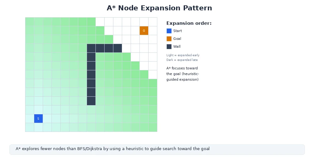
A* is a best-first search algorithm. It explores the grid cell-by-cell, always picking the most promising cell next.
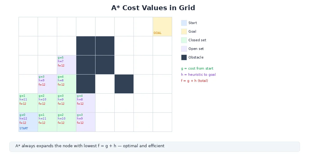
The key insight: For each cell, estimate the total cost to reach the goal through that cell.
f(cell) = g(cell) + h(cell)

where:
  g(cell) = cost to reach this cell from start (known)
  h(cell) = estimated cost from this cell to goal (heuristic)
  f(cell) = estimated total cost (start → cell → goal)
A* always expands the cell with the lowest f(cell). This guarantees it finds the shortest path — as long as the heuristic h(cell) is admissible (never overestimates the true cost).
The A* Algorithm (Step-by-Step)
Let's walk through A* on the grid above.
Setup
- Open set: cells to explore, sorted by
f(cell). Start with just the start cell. - Closed set: cells already explored.
- g-scores: cost to reach each cell from start (initialized to ∞, except start = 0).
- Came-from map: tracks the path (which cell did we come from?).
Loop
while open_set is not empty:
    current = cell in open_set with lowest f(current)

    if current == goal:
        return reconstruct_path(came_from, current)

    remove current from open_set
    add current to closed_set

    for neighbor in neighbors_of(current):
        if neighbor in closed_set:
            continue  # already explored

        tentative_g = g[current] + cost(current, neighbor)

        if tentative_g < g[neighbor]:
            # This path to neighbor is better than any previous one
            came_from[neighbor] = current
            g[neighbor] = tentative_g
            f[neighbor] = g[neighbor] + h(neighbor)

            if neighbor not in open_set:
                add neighbor to open_set
Example Trace
Starting from S at (0, 2), goal G at (5, 2):
Step 1: Expand S. Neighbors: (1,2), (0,1), (0,3). Add to open set.
Step 2: Expand (1,2). Neighbors: (1,1), (1,3), (0,2) already closed. Add (1,1), (1,3).
Step 3: Notice (2,2) is blocked (occupancy = 100). Skip it.
Step 4: Eventually reach (5,2) = G. Reconstruct path from came_from map.
Result: Path is S → (1,2) → (1,1) → (2,1) → (3,1) → (4,1) → (4,2) → (5,2) = G.
The path goes around the wall.
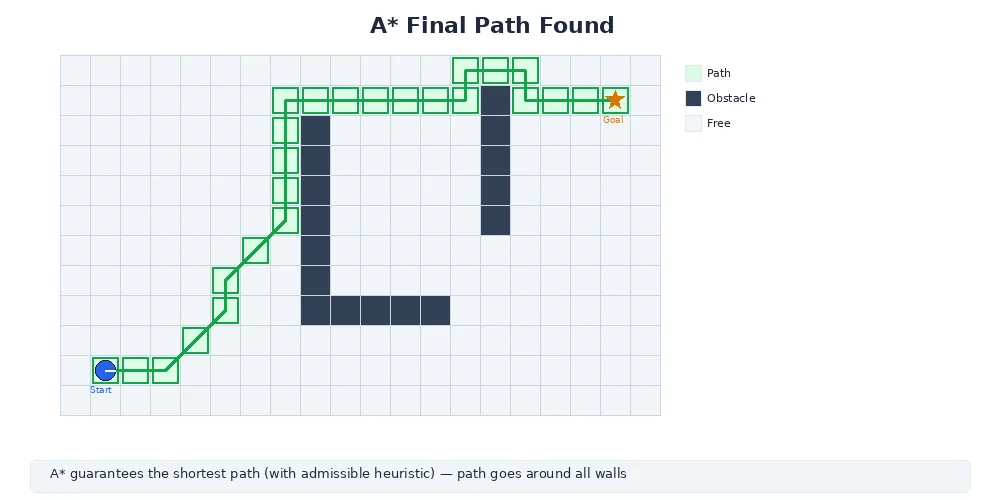
A* is optimal (finds the shortest path) and complete (always finds a path if one exists). Its efficiency depends entirely on the heuristic h(cell). A good heuristic makes A* fast; a bad one makes it slow.
Choosing a Heuristic
The heuristic h(cell) estimates the cost from cell to the goal. Common choices:
| Heuristic | Formula | When to Use |
|---|---|---|
| Euclidean distance | sqrt((x2-x1)² + (y2-y1)²) | Robot can move in any direction (holonomic) |
| Manhattan distance | ` | x2-x1 |
| Diagonal distance | `max( | x2-x1 |
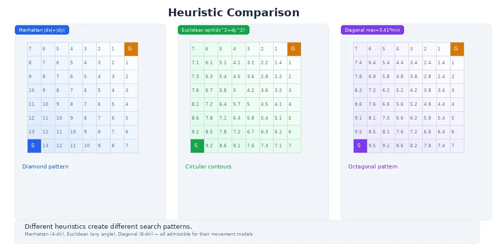
Rule: The heuristic must be admissible (never overestimate) and consistent (h(A) ≤ cost(A→B) + h(B)). Euclidean distance is always safe because it's the straight-line distance — the absolute minimum.
A common mistake: using 0 as the heuristic (h = 0). This turns A* into Dijkstra's algorithm — still correct, but explores many more cells. The heuristic is what makes A* fast.
Cost Functions
The cost cost(current, neighbor) is usually just the distance:
- Straight move (4-way grid): cost = 1.0
- Diagonal move (8-way grid): cost = √2 ≈ 1.414
But you can penalize certain cells:
- Near obstacles: cost = 1.5 (stay away from walls)
- Rough terrain: cost = 2.0 (prefer smooth paths)
- Restricted zones: cost = 10.0 (avoid unless necessary)
This lets you express preferences beyond "shortest distance."
Implementation Notes
from heapq import heappush, heappop
import math

def astar(grid, start, goal):
    open_set = []
    heappush(open_set, (0, start))

    came_from = {}
    g_score = {start: 0}

    while open_set:
        _, current = heappop(open_set)

        if current == goal:
            return reconstruct_path(came_from, current)

        for neighbor in neighbors(current, grid):
            tentative_g = g_score[current] + distance(current, neighbor)

            if tentative_g < g_score.get(neighbor, float('inf')):
                came_from[neighbor] = current
                g_score[neighbor] = tentative_g
                f_score = tentative_g + heuristic(neighbor, goal)
                heappush(open_set, (f_score, neighbor))

    return None  # no path found

def heuristic(a, b):
    # Euclidean distance
    return math.sqrt((a[0] - b[0])**2 + (a[1] - b[1])**2)

def neighbors(cell, grid):
    x, y = cell
    candidates = [(x+1,y), (x-1,y), (x,y+1), (x,y-1)]  # 4-way
    return [c for c in candidates if is_free(c, grid)]
What's Next?
A* works great for 2D maps, but what about high-dimensional spaces like a 6-axis robot arm? Next, we'll explore sampling-based planning — algorithms like RRT that can plan in spaces where grids fail.